Profiling Go Packages: Bipartite Graphs
Package bipartite grew out of another project when the latter’s increasingly complex and poorly modularized code suggested that some refactoring was in order. It’s a small package that implements undirected bipartite graphs. These are graphs whose vertices can be separated into two disjoint and independent sets—the members of each set are connected only with members of the other. Bipartite graphs can model NP-hard problems such as set cover optimization and are used extensively in coding theory and distributed system analysis.
Some useful operations for a bipartite graph data structure:
- Add and remove nodes
- Add and remove edges
- Report a node’s degree (number of edges)
- List a node’s adjacent nodes
- Report the number of nodes in either set
- List the nodes in either set
The first four operations are reasonable expectations of any graph package; the last two are specific to bipartite graphs, and the package’s graph data structure should be designed to accommodate them to the extent possible.
The implementation begins with empty interface types A and B, whose values will represent elements of vertex sets that are of (notionally) distinct dynamic types, and a Graph type which is a struct containing a pair of symmetric maps to hold the adjacency information.
// A is a node that is only adjacent to B nodes.
// Values must be comparable using the == and != operators.
type A interface{}

// B is a node that is only adjacent to A nodes.
// Values must be comparable using the == and != operators.
type B interface{}

// Graph is an undirected bipartite graph.
type Graph struct {
	ab map[A]map[B]struct{}
	ba map[B]map[A]struct{}
}
Under the hood, the Graph type’s maps are a map of As to “sets” of Bs (in the form of a map[B]struct{}1), and a corresponding map of Bs to A “sets”. An (undirected) edge between a node a of type A and a node b of type B is represented internally by the presence of b in a’s set and vice versa.2
func (g *Graph) Add(a A, b B) {
	// Create a node's set if this is its first edge.
	if _, ok := g.ab[a]; !ok {
		g.ab[a] = make(map[B]struct{})
	}
	if _, ok := g.ba[b]; !ok {
		g.ba[b] = make(map[A]struct{})
	}

	// Add a and b to each other's sets.
	g.ab[a][b] = struct{}{}
	g.ba[b][a] = struct{}{}
}
Having two maps, one indexed by As and holding Bs and the other indexed by Bs and holding As, makes it much quicker to determine set membership than, say, a single map indexed by As alone: in the later case, the question of which As are adjacent to a particular B can only be answered by a range loop over the entire map.
Beyond this, however, the distinction is somewhat artificial. Discounting the separate A and B versions of the Deg, N, Remove, and neighbor functions, which could be designed to interface in such a way that only one of each was necessary,Add and Delete are the only functions that actually enforce the bipartite character of the graph, and they only do so to the extent that the caller correctly keeps their set values distinct.
Design variations
The initial implementation certainly suggests a few possible modifications worth investigating.
- Instead of two separate types and two separate maps, why not just one map accepting values of any type?
It would be nice to have to expose only one Deg and Remove function, and one function to replace both of As and Bs (AdjacentTo? Neighbors?). Since A and B are both empty interface types, it would be easy enough to have Graph consist of a single map[interface{}]map[interface{}]struct{}. Now the definition-as-documentation of A and B representing separate sets is lost, and it becomes harder to answer questions like “How many a-type nodes are in the graph?” or “Which bs are in the graph?” without a range loop, unless Graph also records holds a separate record of which keys are present—something like dual map[interface{}]struct{}s for values Added as as and bs. The code would otherwise be slightly simpler, with only one internal map to refer to instead of two, although a symmetric pair of operations would still be required to add or delete an edge. On the other hand, this would invalidate applications in the case that there could exist an element in each set with the same underlying value.3
- The sets could also be defined as maps to boolean values, like
map[interface{}]bool.
The primary disadvantage of using struct{} is that the code gets a little cluttered, particularly the check for set membership: since a map lookup on a key that is not present in the map returns the zero value, lookups in maps that might hold the zero value (like, for example, struct{}{}) require the use of Go’s “comma ok idiom”, which reports whether a map holds a key via the special dual assignment form v, ok := m[k]. This yields an additional untyped boolean value, conventionally called ok, which is true precisely when the key k is present in the map. An alternative would involve storing only non-zero values. The next smallest amount of storage that a value can take up is a single byte, and booleans fit the bill, which is nice because true is not the boolean zero value, and storing it instead of struct{}{} cleans up the adjacency check quite nicely.
// Invalid (always true): map lookups return the zero value
// when the key is absent
if g.ab[a][b] == struct{}{} {

// Valid and idiomatic, but a mouthful
if _, ok := g.ab[a][b]; ok {

// Works with a boolean value type
if g.ab[a][b] {
These two variations can be investigated independently. A final idea, and all but certainly the greatest improvement in terms of clarity and performance, is discussed below in “Next steps” because it’s not a part of the language yet…
Benchmarking
The unit tests in bipartite_test.go use graphs that aren’t any more complicated than necessary to test the package’s edge cases. To simulate a larger and slightly less contrived workload, the benchmark functions operate on a graph mapping the hundred most common English verbs to the letters they contain: 403 edges connecting 100 A nodes, of degrees ranging from 2 (be, do, go, see) to 8 (consider, understand), with 24 B nodes (excluding j and z), of degrees ranging from 1 (q, x) to 59 (e).
$ go test -bench=.
goos: darwin
goarch: amd64
pkg: github.com/dkmccandless/bipartite
BenchmarkNew-4                 	97772346	        11.7 ns/op
BenchmarkAdjacent-4            	16263823	        72.4 ns/op
BenchmarkAdd/create_nodes-4    	  813938	      1354 ns/op
BenchmarkAdd/extant_nodes-4    	 1551062	       778 ns/op
BenchmarkDelete/retain_nodes-4 	 2442205	       480 ns/op
BenchmarkDelete/delete_nodes-4 	 1978154	       613 ns/op
BenchmarkRemoveA-4             	  629308	      1760 ns/op
BenchmarkRemoveB-4             	  156804	      7172 ns/op
BenchmarkAs-4                  	  770144	      1527 ns/op
BenchmarkBs-4                  	 3141134	       404 ns/op
BenchmarkAdjToA-4              	 6847228	       173 ns/op
BenchmarkAdjToB-4              	 2877238	       409 ns/op
BenchmarkDegA-4                	48172159	        25.4 ns/op
BenchmarkDegB-4                	48042222	        26.0 ns/op
BenchmarkNA-4                  	1000000000	         0.255 ns/op
BenchmarkNB-4                  	1000000000	         0.254 ns/op
BenchmarkCopy-4                	    8386	    138592 ns/op
PASS
ok  	github.com/dkmccandless/bipartite	531.204s
Note the similar ratios of roughly 4 to 1 between RemoveA and RemoveB, As and Bs, and to a lesser extent AdjToA and AdjToB. This reflects both the ratio of As to Bs in the graph and the adjacency degrees of the benchmarked nodes, “require” (5) and “r” (24), with the differences due mainly to the time spent allocating space for the slices’ underlying arrays.
And what’s up with NA and NB taking single-digit numbers of clock cycles per operation? Congratulatory messages regarding my benchmarking prowess will be graciously redirected to the Go Authors. What’s actually going on is that the compiler is optimizing the function call away in its entirety: since these functions take no input parameters and have no side effects on any global state, the compiler takes the liberty of speeding up the for loop by eliminating the tedium of actually calling them. From now on, we’ll follow suit; it’s just a simple map length lookup anyway.
Eagle-eyed number buffs might also notice the drastic discrepancy between the total elapsed time displayed at the end of the output and the sums of the individual benchmark durations, each of which is on the order of a second. The culprits are the Add, Delete, and Remove routines, which pause the benchmarking timer to reset the changes to the Graph made by the function being examined. The time cost of b.StopTimer() and b.StartTimer() thoroughly outweighs the duration of the benchmarked functions themselves, but patience is the price of an accurate result. The alternatives would be to reset the Graph’s state with the timer running, rendering the individual benchmarking results meaningless (and to an extent, redundant), or not to reset the state at all, making the results merely a measure of how long it takes to modify the state once and then check that it doesn’t need to be modified a few million times after that.
Here are the results (in nanoseconds) for each design variation side by side.
| Function | Original | Boolean value | Single map | Single map, boolean value |
|---|---|---|---|---|
| New | 11.7 | 11.7 | 15.6 | 17.9 |
| Adjacent | 72.4 | 74.6 | 95.8 | 81.2 |
| Add/create_nodes | 1354 | 1396 | 1460 | 1447 |
| Add/extant_nodes | 778 | 821 | 861 | 851 |
| Delete/retain_nodes | 480 | 526 | 552 | 530 |
| Delete/delete_nodes | 613 | 664 | 838 | 800 |
| RemoveA | 1760 | 1884 | 2965 | 2999 |
| RemoveB | 7172 | 7233 | 10710 | 10753 |
| As | 1527 | 1534 | 1605 | 1597 |
| Bs | 404 | 392 | 399 | 383 |
| AdjToA | 173 | 178 | 171 | 173 |
| AdjToB | 409 | 426 | 442 | 420 |
| DegA | 25.4 | 27.0 | 28.1 | 24.7 |
| DegB | 26.0 | 24.5 | 26.3 | 26.2 |
| Copy | 138592 | 139269 | 160216 | 159377 |
Results are prone to some fluctuation based on background CPU utilization and power management—even with my machine plugged in, shorter benchmark runs (less than a few hundred milliseconds) consistently return slightly faster results than anything longer—so a few percent here or there isn’t very significant. But the correlations are apparent: boolean vs. empty struct times are statistically indistinguishable, perhaps with the exception of Delete. On the other hand, the single map implementations take 10-30% more time than the original dual map configuration, and up to 70% more time in Remove.
Profiling
To dive deeper into these results, let’s examine a new benchmark function that combines a few Graph operations:
func BenchmarkConstructDestruct(b *testing.B) {
	for i := 0; i < b.N; i++ {
		g := New()
		// Add each word in the list as an A node,
		// connected with each of its letters as a B node.
		for _, s := range dict {
			for _, b := range s {
				g.Add(s, string(b))
			}
		}
		for b := 'a'; b <= 'z'; b++ {
			g.Remove(string(b))
		}
	}
}
Construct the graph by Adding a connection between each word and each letter it contains (creating either node when it is passed to Add for the first time), and then Remove each letter node and delete its connections (removing the adjacent word node if this was its last edge).
The -benchmem flag reports average memory usage and allocations in addition to execution time:
$ go test -bench=Construct -benchtime=10s -benchmem
goos: darwin
goarch: amd64
pkg: github.com/dkmccandless/bipartite
BenchmarkConstructDestruct-4   	   34878	    341246 ns/op	   68948 B/op	    1649 allocs/op
PASS
ok  	github.com/dkmccandless/bipartite	15.624s
| Implementation | Time | Memory | Allocations |
|---|---|---|---|
| Original | 341246 ns/op | 68948 B/op | 1649 allocs/op |
| Boolean | 347370 ns/op | 72764 B/op | 1649 allocs/op |
| Single map | 439854 ns/op | 82079 B/op | 1660 allocs/op |
| Single map + boolean | 442439 ns/op | 86458 B/op | 1661 allocs/op |
The -cpuprofile and -memprofile flags instruct the testing command to generate CPU and memory profiles for Go’s pprof tool, which can generate snappy graph summaries of runtime function calls and execution times, as well as flame graphs (three cheers!) to instantly highlight costly call paths.
| Dual map CPU usage | Single map CPU usage |
|---|---|
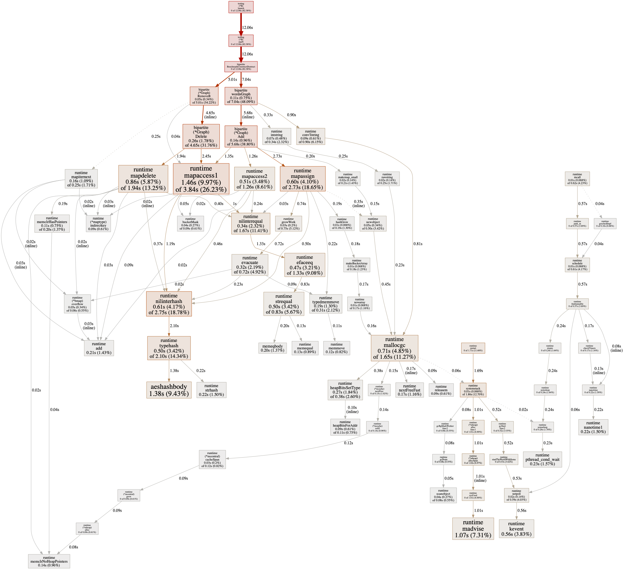 |
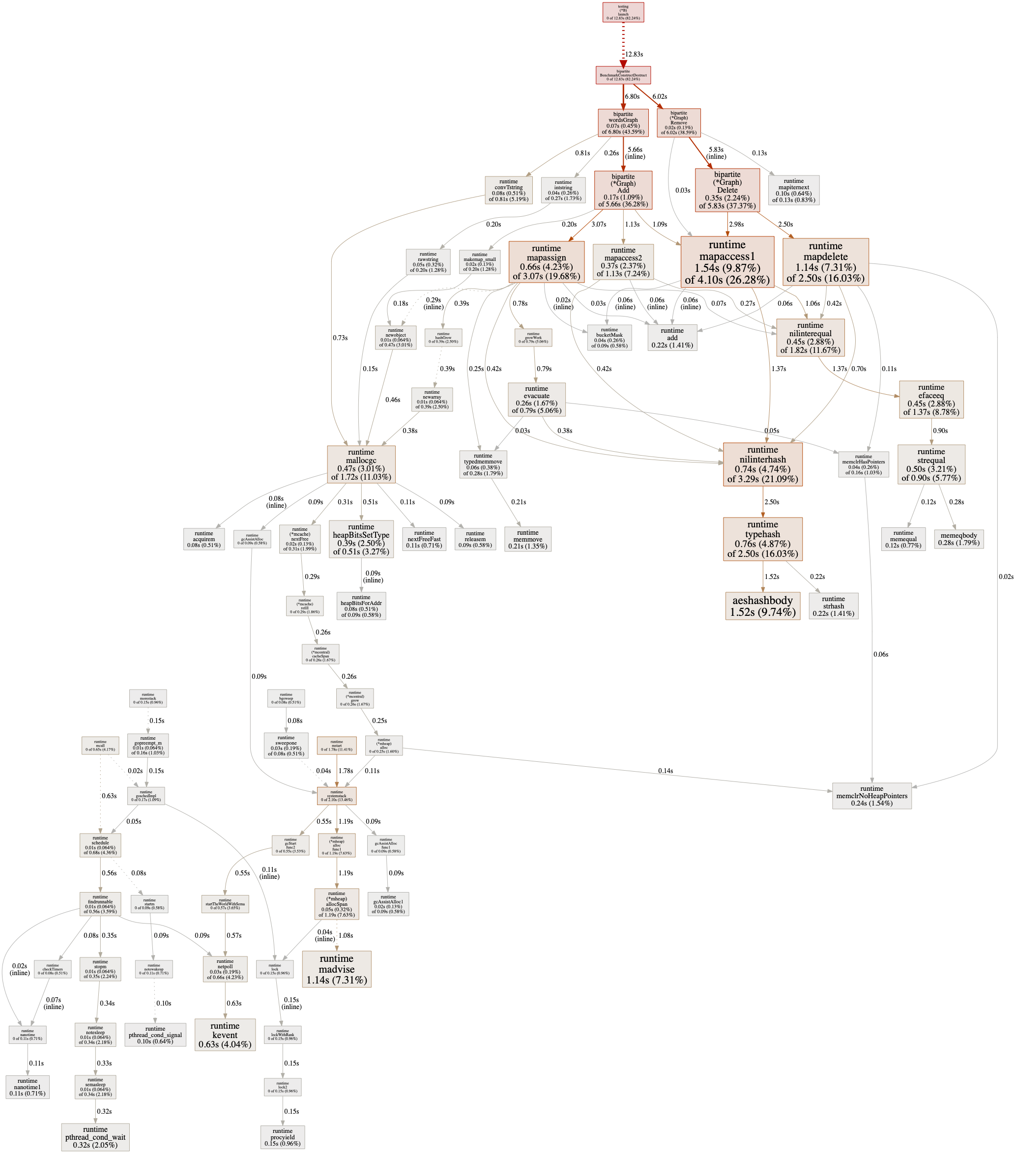 |
Usually, when I’ve generated a pair of these in pursuit of some bit of performance optimization, my first inclination is to either stand far from the screen and view them side by side as an autostereogram or flip between them like a blink comparator to glean their large-scale relationships.
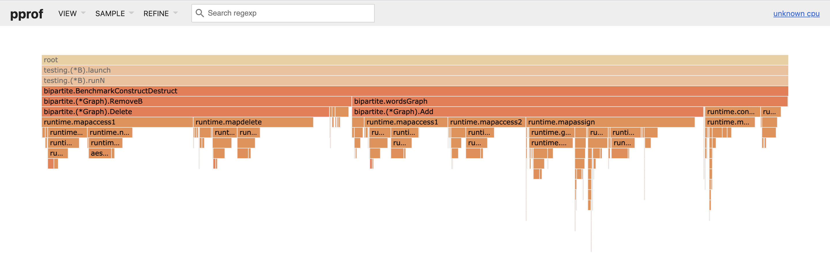
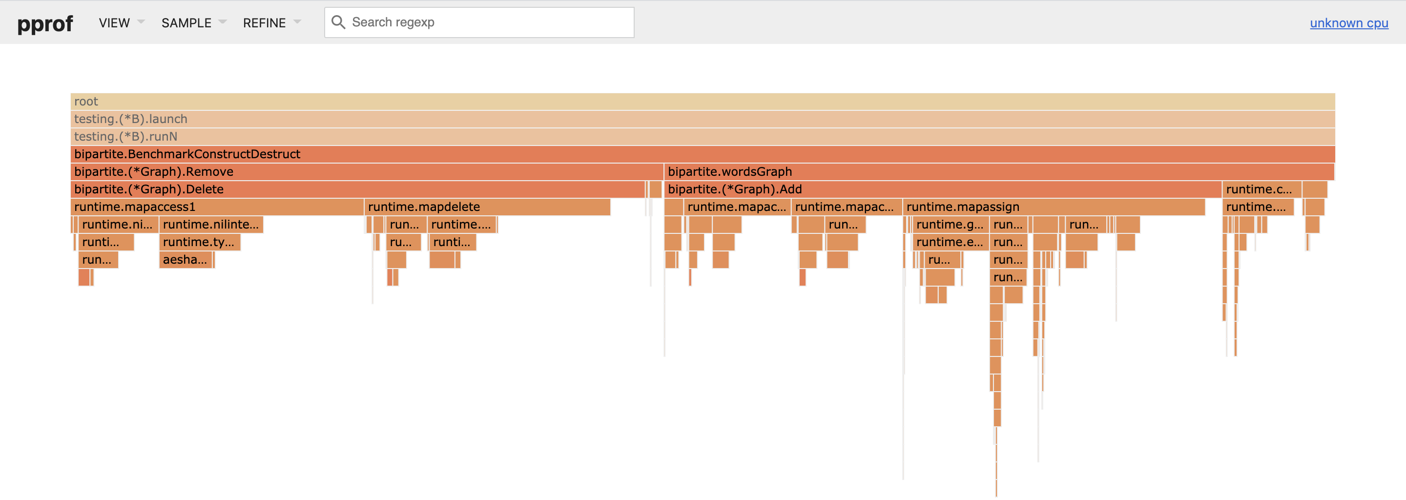
The standout here is Remove, and Delete within it, which takes up 20% more time in the single map profile, in line with the benchmark measurements. It seems reasonable that this has to do with the average-case O(N log N) performance of maps with key types that need to be hashed: with all keys held in a single map, lookups will simply take proportionally longer. There’s a lot more data to pore through in the profiles, and pprof offers more ways to analyze them, but in this case the other differences are all variations on the theme of map operations taking longer in the single map implementation.
Conclusions
The original dual map implementation is an obvious winner. The intended usage is more clearly documented, lookup operations are faster when the maps are smaller, and the very idea of fitting all keys into a single data structure ignores the fact that other data structures are necessary to implement the As and Bs functions anyway. That’s a clear indication that the internal structure of the Graph type should incorporate the bipartite nature of the data. And then there’s the issue of not being able to handle the same value entered as both an A and a B and guarantee that the graph is still bipartite.
This is all because there is already a smart and functional division of labor baked right into the dual map implementation. A weak analogy would be a normalized database: it might look a little more complex on paper, but it’s easier to work with, and behind the scenes it just runs cleaner. (And that complexity, or the simplicity of an alternative, may well turn out to be illusory.)
So dual-map is at least as clear to reason about and easy to document, and its edge cases are fewer and more straightforward. It’s even slightly less code. If single-map had any of these things going in its favor, there would be more to discuss, but the decision is unanimous.
The choice of whether to adopt an empty struct or boolean map value isn’t nearly as clear-cut. Storing true does take more space, although not by much: 84 kilobytes vs. 67, or 19% more memory—significant, if not overwhelming, considering that the bulk of that space is used to encode the graph structure itself (in the form of the nested maps, rather than the values of those maps). And what it didn’t take much more of at all was time.
This is more of a judgment call: in an application where space is at a premium, struct{}{} seems like the way to go. On the other hand, I’d strongly consider map[A]bool/map[B]bool if it made much of a difference to the readability of the codebase—there’s a strong argument for a couple percent of speed/memory being a reasonable price to pay for keeping the code easier to maintain in the long run. In this package’s case, there’s actually only one place outside of the test file that can be rewritten to read more pleasantly with boolean values, in Adjacent:
func (g *Graph) Adjacent(a A, b B) bool {
	if _, ok := g.ab[a]; !ok {
		return false
	}
	// Compare "return g.ab[a][b]"
	_, ok := g.ab[a][b]
	return ok
}
So I think I’ll stick with the empty struct. A byte here, a nanosecond there… Much ado about very little, one might think, but isn’t that the benchmarker’s motto?
Next steps
Of course, in terms of design considerations, it’s still hardly ideal that the exported namespace is so cluttered with As and Bs left and right, most egregiously in the form of otherwise identical interface types. The long-anticipated advent of generics in Go 2 should help a lot with this. Exporting 30% fewer identifiers with clearer documentation and no negative impact on functionality? Sign me up. When the time comes, converting package bipartite to use generics should be an engaging introductory challenge to learn how to reason about the new “type parameter” syntax. Dispensing with the need to handle everything through interfaces will likely be a significiant performance improvement too.
-
Mathematical sets can be represented in Go using a map whose value type is the empty struct
struct{}. The main uses of the empty struct derive from two unusual properties of its valuesstruct{}{}, both consequences of the fact that empty structs can hold no data: first, there is only one such value, and second, they consume no storage space. ↩ -
This reciprocal relationship encodes the undirected character of the graph. Removing this invariant would be one natural route toward a directed graph implementation. ↩
-
More concretely, there is a pernicious bug lurking in the naive translation from the map pair to the single map implementation: if a node is added in one parameter field of
Addand then later again in the opposite parameter field, it will be recorded in both theasandbsset maps. If it isRemoved later, all of its edges will be deleted and it will be removed frommand whichever ofasandbsit was specified as in the call toRemove, but not the other: one ofasorbswill retain an erroneous phantom record of its presence that will invalidate subsequent calls toNA/NBandAs/Bs, which will return non-zero values even when the Graph is empty. In other words, the single map implementation allowsAddto invalidate the very bipartite character of the graph, and the onus is on the user to recognize and avoid this. ↩